3.1 Gibbs Free Energy

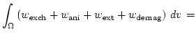
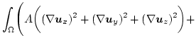
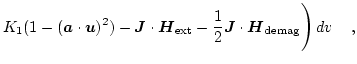
The total Gibbs free energy is given by [33,34]

$$E_\mathrm{tot} = \int_\Omega \left( w_\mathrm{exch}+w_\mathrm{ani}+ w_\mathrm{ext}+w_\mathrm{demag} \right) d{v} =$$ (3.1)

$$= \int_\Omega \Biggl( A \biggl( (\nabla \boldsymbol{u}_x)^2+(\nabla \boldsymbol{u}_y)^2+(\nabla \boldsymbol{u}_z)^2 \biggr)+$$

$$K_1 (1-(\boldsymbol{a} \cdot \boldsymbol{u})^2)- \boldsymbol{J} \... ...1}{2}\boldsymbol{J} \cdot \boldsymbol{H}_\mathrm{demag} \Biggr) d{v} \quad,$$

where

$$\boldsymbol{J}(\boldsymbol{x}, t)=J_\mathrm{s}(\boldsymbol{... ...l{u}(\boldsymbol{x},t) \quad, \quad \vert\boldsymbol{u}\vert=1$$ (3.2)

describes the magnetic polarization as a function of space and time. $A$ is the exchange constant, $K_1$ is the first magnetocrystalline anisotropy constant and $\boldsymbol{a}$ the unit vector parallel to the easy axis, $\boldsymbol{H}_\mathrm{ext}$ the external field, and $\boldsymbol{H}_\mathrm{demag}$ the demagnetizing field.

In thermodynamic equilibrium a micromagnetic system tries to reach a state with minimum total energy. The aim of micromagnetic theory is to find the magnetic polarization in equilibrium. Brown proposed a variational method [33], which is based on the calculation of the variational derivative of the total energy with respect to the magnetic polarization. In equilibrium (in an energy minimum) the coefficients of the linear term vanish for any variation $\delta \boldsymbol{u}$

$$\frac{\delta E_\mathrm{tot}}{\delta \boldsymbol{u}}=0 \quad.$$ (3.3)

This leads to Brown's equations

$$\boldsymbol{u} \times \Bigl( 2 A \Delta \boldsymbol{u} + ... ...hrm{ext}+ J_\mathrm{s}\boldsymbol{H}_\mathrm{demag} \Bigr)=0$$ (3.4)

Thus, in equilibrium the magnetic polarization $\boldsymbol{J}$ is parallel to an ``effective field''

$$\boldsymbol{H}_\mathrm{eff}= \frac{2A}{J_\mathrm{s}} \Delt... ...+ \boldsymbol{H}_\mathrm{ext}+ \boldsymbol{H}_\mathrm{demag}$$ (3.5)

and the torque which acts on the polarization vanishes

$$\boldsymbol{J} \times \boldsymbol{H}_\mathrm{eff}=0 \quad.$$ (3.6)

Since any contribution parallel to the polarization $\boldsymbol{J}$ does not add to the torque, it does not make any difference if the magnetic field $\boldsymbol{H}$ or the magnetic induction $\boldsymbol{B}=\mu_0\boldsymbol{H} + \boldsymbol{J}$ is used for the effective field.