4.1 Energy Minimization

In Sec. 3 we have introduced the Gibbs free energy of a micromagnetic system, discretized various contributions to the total energy, and derived the matrix-vector formulation. Some complication was introduced by the demagnetizing field, but the hybrid finite-element/boundary element method provides an elegant way to solve the problem accurately with a finite element mesh, which is restricted to the magnetic bodies.

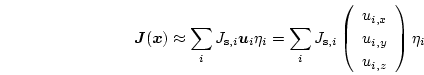
This enables us to implement a simple energy minimization scheme to find the equilibrium magnetization distribution. If the magnetic polarization $\boldsymbol{J}$ is defined in Cartesian coordinates,

$$\boldsymbol{J}(\boldsymbol{x}) \approx \sum_i J_{\mathrm{... ...u_{i,x} \\ u_{i,y} \\ u_{i,z} \end{array} \right) \eta_i$$ (4.1)

one has to use a constrained solver, which ensures, that the norm of $\boldsymbol{J}$ is preserved: $\vert\boldsymbol{J}\vert=J_\mathrm{s}$. However, it has been shown [44,45] that the use of spherical coordinates has several advantages:

• The number of unknowns is reduced by $1/3$, which speeds up the solver.
• The norm is automatically preserved, which allows the use of an unconstrained solver.
• Convergence problems with a Lagrange multiplier approach for the constraint $\vert\boldsymbol{J}\vert=J_\mathrm{s}$ are avoided.

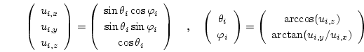
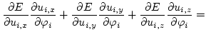
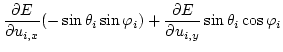
However, the direct calculation of the energy gradient in spherical coordinates causes various problems due to the periodicity of the polar and azimuth angles. Therefore, the magnetic polarization for the minimizer is given in spherical coordinates ( $\theta \in [0;\pi[$, $\varphi \in [0;2\pi[$).

$$\left( \begin{array}{c} u_{i,x} \\ u_{i,y} \\ u_{i,z}... ...os(u_{i,z}) \\ \arctan(u_{i,y}/u_{i,x}) \end{array} \right)$$ (4.2)

Then it is converted to Cartesian coordinates. The energy gradient is calculated in Cartesian coordinates, converted back to spherical coordinates

$$\frac{\partial E}{\partial \theta_i} = \frac{\partial E}{\partial u_{i,x}}\frac{\partial u_{i,x}}{\parti... ...\frac{\partial E}{\partial u_{i,z}}\frac{\partial u_{i,z}}{\partial \theta_i} =$$ (4.3)

$$= \frac{\partial E}{\partial u_{i,x}}\cos\theta_i\cos\varphi _i+ \f... ...,y}}\cos\theta_i\sin\varphi _i- \frac{\partial E}{\partial u_{i,z}}\sin\theta_i$$ (4.4)

$$\frac{\partial E}{\partial \varphi _i} = \frac{\partial E}{\partial u_{i,x}}\frac{\partial u_{i,x}}{\parti... ...rac{\partial E}{\partial u_{i,z}}\frac{\partial u_{i,z}}{\partial \varphi _i} =$$ (4.5)

$$= \frac{\partial E}{\partial u_{i,x}}(-\sin\theta_i\sin\varphi _i)+ \frac{\partial E}{\partial u_{i,y}}\sin\theta_i\cos\varphi _i$$ (4.6)

and returned to the minimizer.

For the minimizer itself the limited memory variable metric (LMVM) algorithm - a quasi-Newton-method - of the TAO package [46,47] has been selected, because it requires only the function values and the gradient of the total energy. In replacement for the Hessian (which is not available due to the demagnetizing field) the second-order information is approximated by a limited history of previous points and gradients. A similar method has been used in [44] and showed better convergence rates than Newton- or Gauß-Seidel methods.