For the direct output of graphics images, the PNG file format has been chosen, because it is widely supported (also by all newer WWW clients), generates very small, highly compressed files, it is not encumbered by any patents (like the GIF file format), and the reference library libpng [66] is freely available.
However, first the magnetization, which is defined on the nodes of the unstructured finite element mesh, has to be interpolated on a regular mesh in the desired slice plane. The slice plane is defined in the configuration file in the form
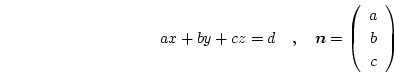 |
(6.1) |
In principle, for each pixel we have to search all tagged elements and determine if the pixel is inside or outside. But we can speed up the search by skipping those elements, for which the distance of the pixel from the first node is larger than the maximum edge length of any tetrahedron.
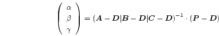
If a suitable element is found we calculate the barycentric coordinates
![]() of the pixel. The barycentric coordinates are defined as the relative position of
of the pixel. The barycentric coordinates are defined as the relative position of ![]() inside the tetrahedron
inside the tetrahedron ![]() . In a ``regular'' tetrahedron (which has three edges coinciding with the coordinate axes) these correspond to the relative coordinates as indicated in Fig. 6.2.
. In a ``regular'' tetrahedron (which has three edges coinciding with the coordinate axes) these correspond to the relative coordinates as indicated in Fig. 6.2.
| (6.2) |
 |
(6.3) |
| (6.4) |
| (6.5) |
The barycentric coordinates
![]() give the weight, by which the data values at the corresponding vertices of the tetrahedron contribute to the linear interpolation at
give the weight, by which the data values at the corresponding vertices of the tetrahedron contribute to the linear interpolation at ![]() . Thus, for some data
. Thus, for some data ![]() defined on the vertices of the tetrahedron, we find the linear interpolation at
defined on the vertices of the tetrahedron, we find the linear interpolation at ![]() with
with
| (6.6) |
As a result we can assemble an interpolation matrix, which calculates the magnetization for all pixels of the image. Let
![]() denote the PETSc vector of one Cartesian component of the magnetization of all nodes of the finite element mesh and
denote the PETSc vector of one Cartesian component of the magnetization of all nodes of the finite element mesh and
![]() the PETSc vector of interpolated values, then we have
the PETSc vector of interpolated values, then we have
| (6.7) |
Since the interpolation matrix depends only on the triangulation, we can calculate it during the initialization phase of the program. Whenever a snapshot of one magnetization component should be stored to disk, a simple matrix-vector multiplication gives the interpolated values at the pixel positions. Then the data are color coded using the scheme shown in Fig. 6.4. Finally, the PNG library [66] is called to convert these data into a PNG graphics file.
In addition to snapshots of the magnetization it is often desirable to measure some data along a probing line through the model. This feature has been implemented based on the algorithm described above. For the probing line we translate and rotate the model to make the probing line coincide with the ![]() -axis. Then we tag all elements, which are cut by the
-axis. Then we tag all elements, which are cut by the ![]() -axis and determine the barycentric coordinates of every point on the sampling line. We finally end up with another interpolation matrix, which calculates the data values along the probing line.
These can then be stored in a data file on disk.
-axis and determine the barycentric coordinates of every point on the sampling line. We finally end up with another interpolation matrix, which calculates the data values along the probing line.
These can then be stored in a data file on disk.
Finally, the complete set of data, which includes the magnetization, the magnetic scalar potential, and the local fields are stored in files in UCD format [75]. This file format can be read by many advanced visualization packages like AVS [76] and MicroAVS [77]. However, the (human-readable) ASCII UCD format generates huge files, because the whole finite element mesh is stored in each file. Thus, two measures have been taken to tackle this problem.
First, the finite element mesh is stored in a single separate file in UCD format during the initialization phase. The data files, which are generated during the simulation are then stored without the mesh definition, which saves about 50% of disk space. Secondly, the data files are compressed using the zlib-library [65] in gzip-compatible format, which shrinks the data to about 30% of their initial size. Thus, we end up with data files, which require only 15% of the uncompressed storage space. To restore the data in proper UCD format, a simple shell script uncompresses the data and merges them with the mesh data. Alternatively, there is also a binary UCD format, which gives smaller files than the standard ASCII format, but it is not as widely supported and may lead to compatiblity problems, when the files are transferred to machines with different hardware architecture and operating system.
![\includegraphics[scale=0.7]{fig/fem/barycent2.eps}](img392.png)
![\includegraphics[scale=0.4]{fig/dots0200651/p1/m22.eps}](img413.png)
![\includegraphics[scale=0.6]{fig/png/color.eps}](img415.png)