2.2 The Weak Formulation

The weak formulation of the boundary value problem $(P)$ is then obtained by the multiplication of Eq. (2.1) with $w \in H_D^1(\Omega):=\{w \in H^1(\Omega)\vert w=0 \mathrm{ on } \Gamma_D\}$ and integration over $\Omega$:

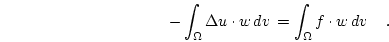$$-\int_\Omega \Delta u \cdot w d{v} = \int_\Omega f \cdot w d{v} \quad.$$ (2.4)

Integration by parts gives

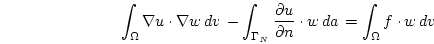$$\int_\Omega \nabla u \cdot \nabla w d{v} - \int_{\Gamm... ...\partial n} \cdot w d{a} = \int_\Omega f \cdot w d{v}$$ (2.5)

and substitution of the boundary conditions and rearrangement leads to

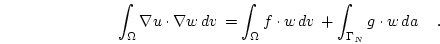$$\int_\Omega \nabla u \cdot \nabla w d{v} = \int_\Omega f \cdot w d{v} + \int_{\Gamma_N} g \cdot w d{a} \quad.$$ (2.6)

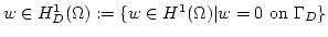
Now we incorporate the (possibly inhomogeneous) Dirichlet boundary conditions

$$\int_\Omega \nabla u \cdot \nabla w d{v} - \int_\Omega... ...t w d{a} - \int_\Omega \nabla u_D \cdot \nabla w d{v}$$ (2.7)

and substitute the homogeneous solution $v \in H^1_D(\Omega)$, which is given by $v=u-u_D$ and satisfies $v=0$ on $\Gamma_D$. This gives us the weak formulation of the Poisson problem $P$ which reads: Find $v \in H^1_D(\Omega)$ such that

$$\int_\Omega \nabla v \cdot \nabla w d{v} = \int_\Omega... ...{a} - \int_\Omega \nabla u_D \cdot \nabla w d{v} \quad.$$ (2.8)