2.4 Mesh Generation

The finite element method requires the discretization of the spatial domain $\Omega$ with ``finite elements'' - a regular triangulation $\mathcal{T}$. For two dimensional problems triangles and rectangles, in three dimensions tetrahedral (cf. Fig. 2.1) and hexahedral elements are commonly used. Also a mixture of different types of elements is possible, but after the evaluation of various other implementations and for simplicity a tetrahedral discretization has been implemented.

Figure 2.1: Kuhn triangulation of a cube into six tetrahedral finite elements (exploded view) [16].

As compared to finite difference methods [17] the finite element mesh may be entirely unstructured, which makes the modeling of complicated geometries and irregular microstructures more convenient. Still, a ``regular'' triangulation of a three dimensional body of arbitrary shape with tetrahedral elements is required to meet several conditions, which have been defined by Ciarlet [18]:

• The nodes of the mesh lie on the vertices of the tetrahedra.
• The elements of the triangulation do not overlap.
• No node lies on an edge of a tetrahedron.
• Each face on the surface of the body belongs either to $\Gamma_D$ or $\Gamma_N$.

If we assume, that the domain $\Omega$ has a surface $\Gamma$ of flat polygons, it is possible to find a triangulation $\mathcal{T}$ with (tetrahedral) finite elements $T$, which cover $\Omega$:

$$\Omega=\bigcup_{T \in \mathcal{T}} T$$ (2.18)

However, the creation of the geometrical model and its triangulation are still very demanding tasks, which require sophisticated (commercial) tools. PATRAN by MSC.SOFTWARE [19] and GID [20] are suitable software packages, which have been used to create the models for this thesis, and for which import filters have been implemented.

The resolution of the finite element mesh - the maximum size of the finite elements - is determined by the smallest features which might occur in the solution of the PDE. These features have to be properly resolved and the approximation of the exact solution by the test functions has to be sufficiently accurate to give meaningful results.

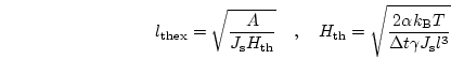
In micromagnetics these limits are defined by three typical lengths:

1. 
   
   $$l_\mathrm{bex}=\sqrt{A/K_1} \quad, \quad \delta_\mathrm{BW}=\pi l_\mathrm{bex}$$
   
   
   $\delta_\mathrm{BW}$ is the width of Bloch type magnetic domain walls (typically found in bulk hard magnets), $A$ is the exchange constant and $K_1$ is the magnetocrystalline anisotropy constant. [21]
2. 
   
   $$l_\mathrm{nex}=\sqrt{2 \mu_0 A/J_\mathrm{s}^2} \quad, \quad \delta_\mathrm{NW}=\pi l_\mathrm{nex}$$
   
   
   $\delta_\mathrm{NW}$ is the width of Néel walls (typically found in soft magnetic materials and thin films), $J_\mathrm{s}$ is the saturation polarization.
3. 
   
   $$l_\mathrm{thex}=\sqrt{\frac{A}{J_\mathrm{s}H_\mathrm{th}}} ... ...rac{2 \alpha k_\mathrm{B} T}{\Delta t \gamma J_\mathrm{s}l^3}}$$
   
   
   $l_\mathrm{thex}$ is the thermal exchange length with the thermal field $H_\mathrm{th}$, which depends on the Gilbert damping constant $\alpha$, the temperature $T$, time step of the numerical time integration scheme $\Delta t$, the gyromagnetic ratio $\gamma$, and the spatial correlation length $l$ (which equals the cell size) [22].

Material parameters of various ferromagnets can be found in App. C in Tab. C.1.

In the most general case, the maximum cell size of the finite element mesh has to be smaller than the minimum of the three lengths defined above [23]. In Sec. 7.3.4 the influence of the mesh size on the pinning field of SmCo permanent magnets is studied in more detail.

However, if the structure of the solution is roughly known, it is possible to use an ``adapted'' mesh for the simulations. It has a high resolution (small elements) in areas with very small features (domain walls) and a low resolution (large elements) in other areas where the solution (magnetization) is very uniform. As a result, the number of nodes (and therefore the number of unknowns) is reduced and the time required for the simulation can be greatly reduced. This technique has been used for the calculation of the equilibrium magnetization distribution in soft magnetic nanodots. The results are presented in Sec. 9.

For dynamic time dependent problems a rigid adapted mesh is often not suitable, because the solution changes over time and the smallest features of the solution move through the mesh. If they leave the high resolution mesh and reach areas with larger finite elements, artificial pinning on the mesh will occur and give wrong results. Thus, an adaptive mesh refinement method is required, which changes the structure of the mesh during the simulation and adapts the resolution of the mesh to the solution. It can be shown, that these methods lead to (almost) optimal complexity and give most accurate results with the smallest numerical (computational) effort [24]. Adaptive mesh refinement methods are still a very active research area, and they have been successfully applied also in numerical micromagnetics [25,26,27,28,29].