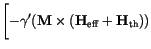
The Milshtein scheme (![]() ) for the stochastic Landau-Lifshitz equation (
) for the stochastic Landau-Lifshitz equation (![]() ) is implemented as
) is implemented as
 |
 |
 |
|
 |
|||
![$\displaystyle -\frac{\alpha \gamma'}{M_\mathrm{s}}
\mathbf{M} \times
(
\mathbf{...
...times (\mathbf{H}_\mathrm{eff} + \mathbf{H}_\mathrm{th})
)
\Biggr]_i
\Delta t +$](img491.gif) |
|||
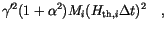 |
(8.1) |
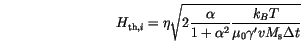
 .
.  is the discretization volume of the computational cells. In the finite difference model it is the volume of a cubic computational cell and in the finite element model it is the volume of the finite element.