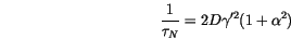
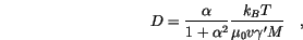
The Fokker-Planck equation, which describes the time evolution of the nonequilibrium probability distribution
 of a set of Langevin equations like (
![]() ), in the Stratonovich interpretation is given by [39]
), in the Stratonovich interpretation is given by [39]
 derivatives of the second term on the right-hand side
 |
 |
 |
|
|
 |
(6.25) |
 |
|
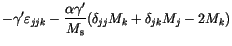
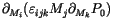
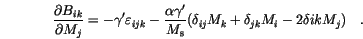
![$\displaystyle \left[
-\gamma'\varepsilon _{ijk} M_j
+\frac{\alpha \gamma'}{M_\m...
...delta_{ik}M^2)
\right]
\left(
-2\frac{\alpha \gamma'}{M_\mathrm{s}} M_k
\right)$](img332.gif) |
|
|
 |
||
|
 |
(6.26) |
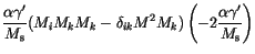
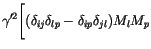
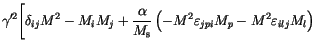
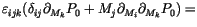
We find, that the second term on the right hand side of (![]() ) vanishes identically. For the third term we find
) vanishes identically. For the third term we find
 |
|
![$\displaystyle \gamma'^2
\Biggl[
-\varepsilon _{ilk} M_l
-\frac{\alpha}{M_\mathrm{s}}
(M_i M_k - \delta_{ik}M^2)
\Biggr] \cdot$](img335.gif) |
|
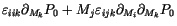
![$\displaystyle \quad \,\, \Biggl[
-\varepsilon _{jpk} M_p
-\frac{\alpha}{M_\mathrm{s}}
(M_j M_k - \delta_{jk}M^2)
\Biggr]
\frac{\partial P}{\partial M_j}$](img336.gif) |
|||
|
 |
||
 |
|||
![$\displaystyle +\frac{\alpha^2}{M^2_\mathrm{s}}
\left(
M^4 \delta_{ik}\delta_{jk...
...delta_{ik}M_j M_k)+
M_i M_j M^2
\right)
\Biggr]
\frac{\partial P}{\partial M_j}$](img339.gif) |
|||
|
 |
||
![$\displaystyle \quad \quad +\frac{\alpha^2}{M^2_\mathrm{s}}
\left(
M^4\delta_{ij}-M^2 M_i M_j
\right)
\Biggr]
\frac{\partial P}{\partial M_j}$](img341.gif) |
|||
|
![$\displaystyle \gamma'^2
\left[
(\alpha^2+1)(M^2 \delta_{ij}-M_i M_j)
\frac{\partial P}{\partial M_j}
\right]$](img342.gif) |
||
|
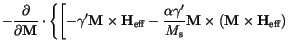
![$\displaystyle -\gamma'^2 (\alpha^2+1)
\left[
\mathbf{M} \times
\left(
\mathbf{M} \times \frac{\partial P}{\partial M_j}
\right)
\right]_i \quad.$](img343.gif) |
(6.27) |
Our result for the Fokker-Planck equation is
is the nonequilibrium probability distribution for  at time
  , and
, and
 stands for the divergence operator
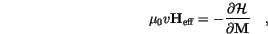
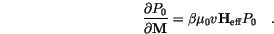
Finally, we have to ensure, that the stationary properties of the stochastic Landau-Lifshitz equation (![]() ), supplemented by the statistical properties of the thermal field (
), supplemented by the statistical properties of the thermal field (![]() ) and (
) and (![]() ), coincide with the appropriate thermal-equilibrium properties. Therefore, the stationary solution of the Fokker-Planck equation
), coincide with the appropriate thermal-equilibrium properties. Therefore, the stationary solution of the Fokker-Planck equation  , for which

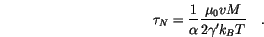
 denotes the discretization volume (the volume of a computational cell) we find
![$\displaystyle \left[
\frac{\partial}{\partial \mathbf{M}} \cdot
\left(
\mathbf{M} \times \frac{\partial P_0}{\partial \mathbf{M}}
\right)
\right]_i$](img356.gif) |
|
||
 |
|
 |
|
|
 |
||
|
 |
(6.31) |
Thus, the Fokker-Planck equation with the stationary solution reads
![\begin{displaymath}
0=\Biggl[
-\frac{\alpha \gamma'}{M_\mathrm{s}}
\mathbf{M}...
...es \beta \mu_0 v \mathbf{H}_\mathrm{eff} P_0
\right)
\Biggr]
\end{displaymath}](img360.gif)
![\begin{displaymath}
\frac{\partial P}{\partial t} =
-\frac{\partial}{\partial ...
...j}
\left[
\left(
D B_{ik}B_{jk}
\right)
P
\right] \quad,
\end{displaymath}](img324.gif)
![\begin{displaymath}
\frac{\partial P}{\partial t} =
-\frac{\partial}{\partial ...
...B_{jk}\frac{\partial}{\partial M_j}
\right) P
\right] \quad.
\end{displaymath}](img326.gif)

![$\displaystyle + \frac{1}{2 \tau_N} \mathbf{M} \times
\left(
\mathbf{M} \times \frac{\partial}{\partial \mathbf{M}}
\right)
\Biggr] P
\Biggr\} \quad,$](img346.gif)