For our problem of calculating the effective field and integrating the Landau-Lifshitz equation, we have to discretize time and space into regular lattices. For the space discretization a regular cubic lattice has been chosen, because it allows the simplest implementation and irregular lattices are more efficiently handled with the finite element method (cf. chapter ![]() ). The time integration is also done on a regular lattice and described in detail in chapter
). The time integration is also done on a regular lattice and described in detail in chapter ![]() .
.
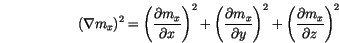
In order to calculate the contribution of the exchange interaction to the effective field, we have to discretize (![]() ). The first partial derivative
). The first partial derivative
 denote the lattice spacing in the three dimensions of space, which is identical on a regular cubic lattice and we will simply write
  .
.
 indicate the finite difference operators in
  and
and  direction, respectively.
Let us now consider the magnetization vector  at lattice point
  and
and
 on the neighbouring lattice point in
  direction. Then, we can rewrite the first term in (
![]() ) as
) as

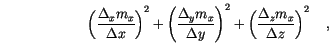
 and component of the magnetization vectors. Since
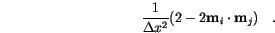
 we can simplify and get for the finite difference
and direction, we get analogous expressions. The same procedure can be carried out for the opposite neighbours in the negative directions of space. Then we take the arithmetic mean of the two opposite nearest neighbours.
we can simplify and get for the finite difference
and direction, we get analogous expressions. The same procedure can be carried out for the opposite neighbours in the negative directions of space. Then we take the arithmetic mean of the two opposite nearest neighbours.
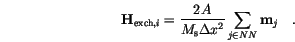
Our final result for the exchange energy density is
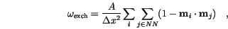 |
(3.3) |
 stands for the indices of the nearest neighbours.
The approximation of the partial derivatives by finite differences is only valid for small arguments, and in our case for small angles between neighbouring magnetization vectors. Other exchange energy representations have been suggested and compared [21], but none of them has significant advantages over the one derived above.
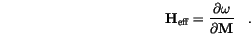
In a discretized form [22] the effective field is defined by
 we find