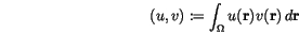
The solution of Poisson's equation (![]() ), which is required to calculate the demagnetizing field
), which is required to calculate the demagnetizing field
 , has to be solved for a given magnetization distribution
 . We write Poisson's equation in a more general form
But first we have to define the vector spaces, in which we are searching for a solution [33]. Given a bounded domain  , we denote by
  the space of quadratically integrable functions defined on . The usual inner product
 and becomes a Hilbert space. The space
  consists of those functions in , whose (weak) derivative of order one also lie in . The
  -inner product is defined as
 belongs to a family of function spaces known as Sobolev spaces. They can be physically interpreted as the space of functions of finite energy with respect to the problem under consideration. In this sense, it is the correct space in which to seek solutions of the weak formulation.
Further, we define the trial space 


 are called test functions.
To derive the weak formulation we multiply Poisson's equation (![]() ) with a test function
) with a test function  and integrate over the solution domain


 denotes the surface normal on the boundary
  . If appropriate boundary conditions define the values of
  (Dirichlet boundary conditions) or of its derivatives
  (Neumann boundary conditions) on the boundary, we can simplify (since
  vanishes, where Dirichlet boundary conditions apply)
The variational formulation of (![]() ) can then be stated in the following general form: Find
) can then be stated in the following general form: Find  such, that
 and the linear functional
  are given by
is sought, becomes equivalent to the test space . Without loss of generality, we can thus assume that we seek the solution in the space . It is noted, that the weak form is a generalization of the classical formulation. Therefore, the solution of the weak formulation need not be a classical solution at the same time.
are given by
is sought, becomes equivalent to the test space . Without loss of generality, we can thus assume that we seek the solution in the space . It is noted, that the weak form is a generalization of the classical formulation. Therefore, the solution of the weak formulation need not be a classical solution at the same time.
Not only Poisson's equation, but a large number of boundary value problems lead to symmetric and positive definite bilinear forms. Also for (![]() ) we find
) we find

 is the sought solution, if it minimizes the functional
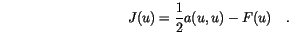
 can often be interpreted as an energy functional.
In the context of Poisson's equation for the demagnetizing field (
can often be interpreted as an energy functional.
In the context of Poisson's equation for the demagnetizing field ( in the magnetic field
 reduces
  to the stray field energy
  and makes equal to the self demagnetizing field
[34].
and makes equal to the self demagnetizing field
[34].
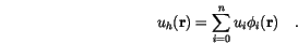
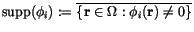
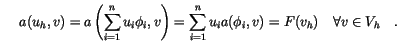
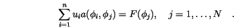
In general, the trial and test space is too large and complex to deal with numerically. Thus, the Galerkin discretization seeks an approximation of the solution  by restricting it to a finite dimensional subspace
  . We rewrite the weak formulation (
![]() ) as follows: Find such, that
) as follows: Find such, that
 shall be approximated by a linear combination of trial functions
 from a finite dimensional subspace of
 lies in , relation (
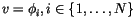 . Conversely, if relation (, then it also holds for all
  . Hence it is sufficient to determine the coefficients
  of
of  such, that
The finite element method is a particular Galerkin method [35], which uses piecewise polynomial functions to construct the finite dimensional subspace . The solution domain is divided into many small subdomains, referred to as elements. In two space dimensions these elements are usually triangles (fig. ![]() ) or convex quadrilaterals, while in three dimensions tetrahedra, prisms and hexahedra are commonly employed. This subdivision process is usually called triangulation. The collection of all elements is referred to as the finite element mesh or grid.
) or convex quadrilaterals, while in three dimensions tetrahedra, prisms and hexahedra are commonly employed. This subdivision process is usually called triangulation. The collection of all elements is referred to as the finite element mesh or grid.
In the finite element method the basis functions
 (fig.
(fig. ![]() ) are chosen in such a way, that
) are chosen in such a way, that
 of each basis function, i.e. the closure of the set, where is nonzero, is small in the sense, that it consists of only a few (connected) elements. (fig. has a simple description in terms of
  so called degrees of freedom which uniquely characterize . Each basis function is characterized by possessing exactly one nonvanishing degree of freedom.
As the support is restricted to a very small local area, the integrals occurring in (![]() ) need only be computed over the small support of each basis function. In fact, most of the integrals are zero, and so the matrix of the linear system of algebraic equations is very sparse.
) need only be computed over the small support of each basis function. In fact, most of the integrals are zero, and so the matrix of the linear system of algebraic equations is very sparse.
|
[Support of basis function ]
![\includegraphics[scale=0.25]{fig/Ex1.5.eps}](img185.gif) [Support of basis function
[Support of basis function  ] ]
![\includegraphics[scale=0.25]{fig/Ex1.6.eps}](img186.gif) [Common support of and ]
[Common support of and ]
![\includegraphics[scale=0.25]{fig/Ex1.7.eps}](img187.gif)
|


![\includegraphics[scale=0.4]{fig/Ex1.0.eps}](img177.gif) [Triangulation]
[Triangulation]
![\includegraphics[scale=0.4]{fig/Ex1.1.eps}](img178.gif)
![\includegraphics[scale=0.6]{fig/Ex1.3.eps}](img182.gif) [Nodal basis function
[Nodal basis function ![\includegraphics[scale=0.6]{fig/Ex1.4.eps}](img184.gif)