4.2 The open boundary problem

For the solution of partial differential equations like Poisson's equation (), we need boundary conditions to find the physically relevant solution. There are three types of boundary conditions:

Dirichlet boundary conditions

The value of the solution is explicitly defined on the boundary of the solution domain (or part of it). The magnetic scalar potential is usually set to zero along a boundary, which should not be crossed by magnetic flux.

Neumann boundary conditions

The normal derivative of the solution is defined on the boundary. If we set the normal derivative of the magnetic scalar potential to zero, the boundary can be interpreted as an interface with a highly permeable metal. Then, the magnetic flux passes the interface at an angle of $90^\circ$ to the plane of the interface. In order to find a unique solution, a Dirichlet boundary condition must be defined somewhere on the boundary of the domain.

Robin boundary conditions

This is a combination of the first two. The solution and its derivative are connected by a given function.

Asymptotic boundary conditions

For many problems neither of the three boundary conditions above is suitable: Natural boundary conditions usually set the solution to a distinct value at infinity. However, finite element methods, can only handle finite domains to solve the problem in a computer at finite speed with finite memory.

One workaround is the truncation of outer boundaries. At an arbitrary distance ``far enough away'' from the area of interest Dirichlet or Neumann boundary conditions are applied. This is very simple, but not very accurate. In addition, it is quite inefficient, because a volume of air, which is much larger than the area of interest, has to be modeled. A fine mesh in the area of interest and a coarse mesh in the exterior can reduce the computational effort again.

Asymptotic boundary conditions transform natural boundary conditions into Robin boundary conditions on the surface of a finite domain. This is achieved by developing the solution into a series expansion of spherical harmonics. Only the leading harmonic is considered, since higher order harmonics decay very quickly.

Hybrid FE/Boundary element method

For the calculation of the magnetic scalar potential the problem of natural boundary conditions applies. Asymptotic boundary conditions require about ten times as many elements for the exterior as for the interior of the magnetic body to obtain a sufficient accuracy [36]. A hybrid finite element/boundary element method combines the advantages of the finite element method (sparse matrices) with those of the boundary element method (no triangulation of the exterior required).

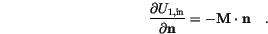
We only know the condition for the potential at the interface between the magnetic body and its surroundings (). The idea of Fredkin and Koehler [37] was to split the magnetic scalar potential $U$ into two parts $U=U_1+U_2$. The potential $U_1$ must satisfy Poisson's equation

$$\Delta U_{1,\mathrm{in}}=\nabla \cdot \mathbf{M}$$ (4.8)

inside the magnetic body and it is set to zero outside.

$$U_{1,\mathrm{out}}=0 \quad.$$

The boundary condition on the surface of the magnet (with surface normal $\mathbf{n}$) is

$$\frac{\partial U_{1,\mathrm{in}}}{\partial \mathbf{n}}=-\mathbf{M} \cdot \mathbf{n} \quad.$$ (4.9)

$U_2$ must satisfy Laplace's equation

$$\Delta U_{2,\mathrm{in}}=0 , \quad \Delta U_{2,\mathrm{out}}=0$$ (4.10)

both, inside and outside the magnetic body. For $U_2$ we find the boundary condition

$$\frac{\partial U_{2,\mathrm{in}}}{\partial \mathbf{n}}= \frac{\partial U_{2,\mathrm{out}}}{\partial \mathbf{n}}$$

and

$$U_{2,\mathrm{out}}-U_{2,\mathrm{in}}=U_{1,\mathrm{in}} \quad,$$

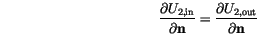
which is required by the continuity of the potential $U$. If we apply the superposition principle, we find, that $U=U_1+U_2$ satisfies () and () and also the boundary condition () is fulfilled.

Since () is a simple Neumann boundary condition, we can calculate $U_1$ from the Poisson equation () with the standard finite element method. The potential $U_2$ is equivalent to the potential of a plane of dipoles with moment $U_1,\mathrm{in}$. Hence, the boundary values of $U_1$ deliver $U_2$ directly by the boundary integral

$$U_2(\mathbf{r})= \frac{1}{4 \pi} \int \frac{U_1(\mathbf{... ...r}')}{(\mathbf{r} - \mathbf{r}')^3} \,d{\mathbf{n}}\, \quad.$$

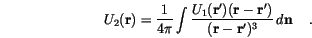In order to save memory, $U_2$ is evaluated only on the surface of the magnet. These values are used as Dirichlet boundary conditions for the solution of the Laplace equation ().